Method

This section gives an overview of the numerical method implemented in ElasticFDSG. For a comprehensive treatment of related subjects readers are referred to Virieux (1986), Levander (1988), and Komatitsch & Martin (2007).

Governing equations

Elastic wave propagation in a linear anisotropic medium is governed by the first-order velocity–stress system:

\[\begin{aligned} \rho \, \partial_t v_x &= \partial_x \sigma_{xx} + \partial_y \sigma_{xy} + \partial_z \sigma_{xz} \\ \rho \, \partial_t v_y &= \partial_x \sigma_{xy} + \partial_y \sigma_{yy} + \partial_z \sigma_{yz} \\ \rho \, \partial_t v_z &= \partial_x \sigma_{xz} + \partial_y \sigma_{yz} + \partial_z \sigma_{zz} \end{aligned}\]

\[\begin{aligned} \partial_t \sigma_{xx} &= C_{11}\,\partial_x v_x + C_{12}\,\partial_y v_y + C_{13}\,\partial_z v_z \\ \partial_t \sigma_{yy} &= C_{12}\,\partial_x v_x + C_{22}\,\partial_y v_y + C_{23}\,\partial_z v_z \\ \partial_t \sigma_{zz} &= C_{13}\,\partial_x v_x + C_{23}\,\partial_y v_y + C_{33}\,\partial_z v_z \\ \partial_t \sigma_{xy} &= C_{66}\!\left(\partial_x v_y + \partial_y v_x\right) \\ \partial_t \sigma_{xz} &= C_{55}\!\left(\partial_x v_z + \partial_z v_x\right) \\ \partial_t \sigma_{yz} &= C_{44}\!\left(\partial_y v_z + \partial_z v_y\right) \end{aligned}\]

The nine independent stiffness coefficients $C_{11}, C_{12}, C_{13}, C_{22}, C_{23}, C_{33}, C_{44}, C_{55}, C_{66}$ describe the most general symmetry supported: orthorhombic (ORT).

Stiffness from Tsvankin parameters

For 3D models, the stiffness tensor is assembled from the Tsvankin parameterisation:

\[\begin{aligned} C_{33} &= V_{P0}^2 \, \rho \\ C_{55} &= V_{S0}^2 \, \rho \\ C_{11} &= (2\varepsilon_2 + 1)\,C_{33} \\ C_{22} &= (2\varepsilon_1 + 1)\,C_{33} \\ C_{66} &= (2\gamma_1 + 1)\,C_{55} \\ C_{44} &= C_{66} / (1 + \gamma_2) \\ C_{13} &= \sqrt{2C_{33}(C_{33}-C_{55})\,\delta_2 + (C_{33}-C_{55})^2} - C_{55} \\ C_{23} &= \sqrt{2C_{33}(C_{33}-C_{44})\,\delta_1 + (C_{33}-C_{44})^2} - C_{44} \\ C_{12} &= \sqrt{2C_{11}(C_{11}-C_{66})\,\delta_3 + (C_{11}-C_{66})^2} - C_{66} \end{aligned}\]

VTI and isotropic models are special cases that can be constructed by the appropiate choice of Tsvankin parameter (see User Guide). For 2D models the standard Thomsen parameterisation is used instead ($\epsilon$, $\delta$).

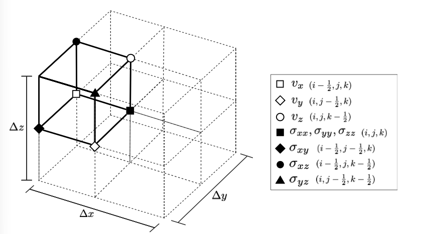
Staggered-grid discretisation

Field components are not co-located but distributed across the unit cell following the standard staggered-grid layout of Virieux (1986). The diagram below shows the elementary cell with all 9 field components placed at their staggered positions:

The discrete leapfrog scheme advances velocities and stresses alternately at half-integer time steps.

Velocity updates (evaluated at staggered positions, using stresses at time $n$):

\[\begin{aligned} v_{x}^{n+\frac{1}{2}}\big|_{(i-\frac{1}{2},\,j,\,k)} &= v_{x}^{n-\frac{1}{2}}\big|_{(i-\frac{1}{2},\,j,\,k)} + \frac{\Delta t}{\rho_{(i-\frac{1}{2},j,k)}} \Big(\partial_x\sigma_{xx} + \partial_y\sigma_{xy} + \partial_z\sigma_{xz}\Big)\Big|_{(i-\frac{1}{2},\,j,\,k)}^{n} \\[6pt] v_{y}^{n+\frac{1}{2}}\big|_{(i,\,j-\frac{1}{2},\,k)} &= v_{y}^{n-\frac{1}{2}}\big|_{(i,\,j-\frac{1}{2},\,k)} + \frac{\Delta t}{\rho_{(i,j-\frac{1}{2},k)}} \Big(\partial_x\sigma_{xy} + \partial_y\sigma_{yy} + \partial_z\sigma_{yz}\Big)\Big|_{(i,\,j-\frac{1}{2},\,k)}^{n} \\[6pt] v_{z}^{n+\frac{1}{2}}\big|_{(i,\,j,\,k-\frac{1}{2})} &= v_{z}^{n-\frac{1}{2}}\big|_{(i,\,j,\,k-\frac{1}{2})} + \frac{\Delta t}{\rho_{(i,j,k-\frac{1}{2})}} \Big(\partial_x\sigma_{xz} + \partial_y\sigma_{yz} + \partial_z\sigma_{zz}\Big)\Big|_{(i,\,j,\,k-\frac{1}{2})}^{n} \end{aligned}\]

Stress updates (evaluated at staggered positions, using velocities at time $n+\frac{1}{2}$):

\[\begin{aligned} \sigma_{xx}^{n+1}\big|_{(i,j,k)} &= \sigma_{xx}^{n}\big|_{(i,j,k)} + \Delta t\Big(C_{11}\,\partial_x v_x + C_{12}\,\partial_y v_y + C_{13}\,\partial_z v_z\Big)\Big|_{(i,j,k)}^{n+\frac{1}{2}} \\[4pt] \sigma_{yy}^{n+1}\big|_{(i,j,k)} &= \sigma_{yy}^{n}\big|_{(i,j,k)} + \Delta t\Big(C_{12}\,\partial_x v_x + C_{22}\,\partial_y v_y + C_{23}\,\partial_z v_z\Big)\Big|_{(i,j,k)}^{n+\frac{1}{2}} \\[4pt] \sigma_{zz}^{n+1}\big|_{(i,j,k)} &= \sigma_{zz}^{n}\big|_{(i,j,k)} + \Delta t\Big(C_{13}\,\partial_x v_x + C_{23}\,\partial_y v_y + C_{33}\,\partial_z v_z\Big)\Big|_{(i,j,k)}^{n+\frac{1}{2}} \\[4pt] \sigma_{xy}^{n+1}\big|_{(i-\frac{1}{2},\,j-\frac{1}{2},\,k)} &= \sigma_{xy}^{n}\big|_{(i-\frac{1}{2},\,j-\frac{1}{2},\,k)} + \Delta t\,C_{66}\Big(\partial_x v_y + \partial_y v_x\Big)\Big|_{(i-\frac{1}{2},\,j-\frac{1}{2},\,k)}^{n+\frac{1}{2}} \\[4pt] \sigma_{xz}^{n+1}\big|_{(i-\frac{1}{2},\,j,\,k-\frac{1}{2})} &= \sigma_{xz}^{n}\big|_{(i-\frac{1}{2},\,j,\,k-\frac{1}{2})} + \Delta t\,C_{55}\Big(\partial_x v_z + \partial_z v_x\Big)\Big|_{(i-\frac{1}{2},\,j,\,k-\frac{1}{2})}^{n+\frac{1}{2}} \\[4pt] \sigma_{yz}^{n+1}\big|_{(i,\,j-\frac{1}{2},\,k-\frac{1}{2})} &= \sigma_{yz}^{n}\big|_{(i,\,j-\frac{1}{2},\,k-\frac{1}{2})} + \Delta t\,C_{44}\Big(\partial_y v_z + \partial_z v_y\Big)\Big|_{(i,\,j-\frac{1}{2},\,k-\frac{1}{2})}^{n+\frac{1}{2}} \end{aligned}\]

The central difference operators for accuracy order $N$ with coefficients $k_l$ are:

\[\begin{aligned} \partial_x f\big|_{(i,j,k)} &\approx \sum_{l=1}^{N} \frac{k_l}{\Delta x} \Bigl(f_{(i+l,\,j,\,k)} - f_{(i-l,\,j,\,k)}\Bigr) \\[4pt] \partial_y f\big|_{(i,j,k)} &\approx \sum_{l=1}^{N} \frac{k_l}{\Delta y} \Bigl(f_{(i,\,j+l,\,k)} - f_{(i,\,j-l,\,k)}\Bigr) \\[4pt] \partial_z f\big|_{(i,j,k)} &\approx \sum_{l=1}^{N} \frac{k_l}{\Delta z} \Bigl(f_{(i,\,j,\,k+l)} - f_{(i,\,j,\,k-l)}\Bigr) \end{aligned}\]

The combination of staggered spatial and temporal grids yields second-order accuracy in both space and time, $\mathcal{O}(\Delta t^2,\, \Delta x^{2N})$.

Note that since density $\rho$ and stiffness $C_{ij}$ are defined at integer nodes, effective values at staggered positions are obtained by averaging neighboring grid points, introducing a non-physical smoothing of material discontinuities.

Domain extension

Starting from the user-defined physical domain of size $n_x \times n_y \times n_z$, the grid is extended in two stages:

1. PML layers — $N_\mathrm{PML}$ absorbing cells appended at each absorbing boundary.
2. Ghost nodes — $N_g = N$ additional cells beyond the PML to support the finite-difference stencil at every interior point.

Material properties in the extended region are filled by nearest-neighbour replication from the physical domain.

Absorbing boundaries — C-PML

Without absorbing boundaries, waves reflect off the computational domain edges. ElasticFDSG uses the convolutional perfectly matched layer (C-PML) of Komatitsch & Martin (2007), which replaces each spatial derivative $\partial_x$ with the modified operator:

\[\tilde{\partial}_x f = \partial_x f + \psi_x\]

where $\psi_x$ is a memory variable updated each time step:

\[\psi_x^{n+1} = b_x \, \psi_x^{n} + a_x \, \partial_x f^{n+1}\]

The precomputed coefficients are:

\[b_x = \exp\!\bigl(-(d_x + \alpha_x)\Delta t\bigr), \qquad a_x = \frac{d_x}{d_x + \alpha_x}(b_x - 1)\]

The damping profile $d_x$ increases polynomially from zero at the physical/PML interface to a maximum at the outer boundary, while the frequency-shift parameter $\alpha_x$ is set to $\pi f_\mathrm{dom}$. This formulation requires 18 additional memory variables in 3D (6 per spatial direction), stored only inside the PML region.

Moment tensor source

Sources are injected as incremental stresses following Shi et al. (2018). The source time function derivative $\dot{s}(t)$ is scaled by the scalar seismic moment $M_0$ and distributed over the stress components:

\[\sigma_{xx(i,j,k)}^{n+1} \mathrel{-}= \frac{\Delta t}{\Delta x \Delta y \Delta z} M_0 \hat{M}_{xx} \dot{s}(t_{n+1})\]

The normal stress components are applied at a single node $(i,j,k)$. Each shear component is symmetrically distributed over four neighboring nodes:

\[\sigma_{xy(I)}^{n+1} \mathrel{-}= \frac{\Delta t}{4 \Delta x \Delta y \Delta z} M_0 \hat{M}_{xy} \dot{s}(t_{n+1}), \quad I = \!\left(i{\pm}\tfrac{1}{2},\, j{\pm}\tfrac{1}{2},\, k\right)\]

(and analogously for $\sigma_{xz}$ and $\sigma_{yz}$). This symmetric distribution produces the correct radiation pattern for each moment tensor configuration.

Moment tensor from fault geometry

For shear-slip (double-couple) sources, the moment tensor components can be computed from strike $\Phi$, dip $\delta$, and rake $\lambda$ (coordinate system: $x$→ North, $y$→ East, $z$↓):

\[\begin{aligned} M_{xx} &= -\!\bigl(\sin\delta\cos\lambda\sin 2\Phi + \sin 2\delta\sin\lambda\sin^2\!\Phi\bigr) \\ M_{yy} &= \phantom{-}\sin\delta\cos\lambda\sin 2\Phi - \sin 2\delta\sin\lambda\cos^2\!\Phi \\ M_{zz} &= \phantom{-}\sin 2\delta\sin\lambda \\ M_{xy} &= \phantom{-}\sin\delta\cos\lambda\cos 2\Phi + \tfrac{1}{2}\sin 2\delta\sin\lambda\sin 2\Phi \\ M_{xz} &= -\!\bigl(\cos\delta\cos\lambda\cos\Phi + \cos 2\delta\sin\lambda\sin\Phi\bigr) \\ M_{yz} &= -\!\bigl(\cos\delta\cos\lambda\sin\Phi - \cos 2\delta\sin\lambda\cos\Phi\bigr) \end{aligned}\]

Receivers

Geophones

Point receivers record the three particle velocity components $v_x$, $v_y$, $v_z$ at each time step. Due to the staggered arrangement, each component is sampled at its natural staggered grid location (offset by half a cell from the nominal receiver position).

DAS

Distributed acoustic sensing (DAS) receivers record axial strain along coordinate-aligned profiles. Within the staggered-grid framework, strain can be reconstructed from the co-located normal stress components via the compliance relation:

\[\begin{bmatrix} \varepsilon_{xx} \\ \varepsilon_{yy} \\ \varepsilon_{zz} \end{bmatrix} = \begin{bmatrix} C_{11} & C_{12} & C_{13} \\ C_{12} & C_{22} & C_{23} \\ C_{13} & C_{23} & C_{33} \end{bmatrix}^{-1} \begin{bmatrix} \sigma_{xx} \\ \sigma_{yy} \\ \sigma_{zz} \end{bmatrix}\]

The axial strain component along the fiber orientation is extracted from the resulting vector. Gauge-length integration or conversion to strain rate can be performed in post-processing. Only fibers aligned with the $x$-, $y$-, or $z$-axis are supported.

References

• Virieux, J. (1986). P-SV wave propagation in heterogeneous media: Velocity-stress finite-difference method. Geophysics, 51(4), 889–901.
• Levander, A. R. (1988). Fourth-order finite-difference P-SV seismograms. Geophysics, 53(11), 1425–1436.
• Komatitsch, D., & Martin, R. (2007). An unsplit convolutional perfectly matched layer improved at grazing incidence for the seismic wave equation. Geophysics, 72(5), SM155–SM167.
• Shi, P., Angus, D., Nowacki, A., Yuan, S., & Wang, Y. (2018). Microseismic full waveform modeling in anisotropic media with moment tensor implementation. Surveys in Geophysics, 39, 567–611.
• Bécache, E., Fauqueux, S., & Joly, P. (2003). Stability of perfectly matched layers, group velocities and anisotropic waves. Journal of Computational Physics, 188(2), 399–433.